Detecting Bottlenecks in Deep RL, Part 2: Sampling

Summary

• Sampling bottlenecks are one source of regret, a measure of how much the agent underperforms an optimal agent throughout training.
• If we can isolate this source from other sources of regret, we would know how much sampling limits training.
• Naively, if all other aspects of our agent are perfect, then all regret is due to sampling.
• I discuss some methods for estimating this sampling regret for different MDP types.

Bottlenecks Recap

In the first post of this blog series, I discussed how bottlenecks in different elements of an RL agent will limit the performance of the whole system. If we can detect and remove these bottlenecks, our RL agents should perform much better on the tasks we are interested in.

Removing bottlenecks happens all the time in applied RL, but it’s something of an ad-hoc process that’s a big part of the “black magic” of RL research. The more structure we can provide, the more we can reduce this process to a practice rather than an art.

To that end, this blog post is about methods for detecting bottlenecks in RL agents, a topic which (to my knowledge) hasn’t been explicitly described anywhere before. The goal is to define metrics of an agent’s performance which can be used by a human researcher to diagnose which factors are performance-limiting so they can be improved upon via various methods. In essence, how do we identify the practical limitations of our algorithms?

Since different parts of an RL algorithm will show their limitations in different ways, this topic is broad and I decided to break up the discussion based on the aspect of the RL agent being considered. This post is gonna focus specifically on sampling-related bottlenecks, since that’s the case I’m most familiar with from my research.

How to Measure Sampling?

In RL, sampling is always going to limit the rate the agent learns. We can imagine that a “perfect training set” exists for any given agent, which consists of the sequence of experiences (presented in precisely the right order) which will make the agent converge to the optimal policy the fastest*. Of course, any sampling strategy (or offline dataset of pre-collected experiences) will fall short of that ideal, so more practically we would like to reason about how much room for improvement there is in the data being collected by our agent, with the knowledge that we will never achieve perfect sampling.

Sidenote: Throughout this blog post I’m mostly gonna talk about things in terms of online RL, where we are trying to optimize the set of trajectories our policy samples over time, such that the policy converges faster to the optimal policy (fewer sub-optimal trajectories sampled, or at least those trajectories should yield better returns). The same considerations can be made for offline RL, where we might want to optimize either a much smaller set of online trajectories (used for rapid fine-tuning to new tasks) or an offline set of trajectories (to improve 0-shot performance on the evaluation tasks). I’ll leave discussion of offline methods to another blog post, since optimizing offline static datasets touches on a lot of other topics.

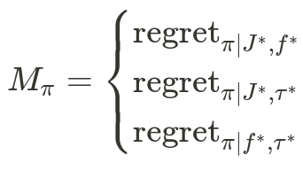
So, how can we measure the quality of our sampling strategy? In theoretical/non-deep RL it’s common to talk about regret minimization, where we want our agent to minimize the difference between the expected return of the agent and the expected return of an optimal agent, cumulatively across training:

where N is the total number of policy improvement steps and pi_i indicates the policy after i iterations of training (sampling+policy update).

A perfect RL agent would thus have 0 regret, as it can (magically) learn the task instantly. Regret then lets us measure how close to perfect our agent is, keeping in mind that perfect is unachievable in practice.

In deep RL, we can compute regret only if we know the value of the optimal policy, which we don’t in general. In practice however we often have a good prior estimate of it for most tasks*. That said, regret measures the total sub-optimality of an RL agent and it’s training process, but doesn’t differentiate between sub-optimality due to different causes- an agent could have high regret due to a poor learning algorithm (e.g. naive REINFORCE), or due to a bad sampling strategy (e.g. greedy sampling).

The challenge, then, is to develop an algorithm that can tell us what fraction of our sub-optimality is due to sampling versus learning algorithm versus model architecture.

Imagine that we had an RL agent which can compute perfect policy gradients (the best possible update for the given data) and has a model with infinite representational capacity. The regret of that model, if non-zero, must be due to sampling/limited data, yes? Similarly, we can imagine an RL agent where our data is perfect and our model has infinite capacity, but we’re stuck with mere mortal methods for updating our policy. Following the pattern, there’s also the third case, where our data is perfect and we have perfect updates, but our model has limited representational power.

This gives is a set of metrics to develop: If we can measure the hypothetical performance of our agent when other aspects are perfect, we can tell how much of a bottleneck the imperfect aspect is for learning. I’ll cover the other cases in future blog posts, but for now let’s concern ourselves with that first case, regret given perfect update rule and model function.

Let’s give this metric a name: I’ll call it Sampling Regret for now. Naively, sampling regret is the regret of an RL agent which is a perfectly efficient learner- the agent can always synthesize the best policy possible from a given set of experiences. For the simplest case of a deterministic MDP with a discrete state space (e.g. tabular RL), this perfectly efficient learner simply remembers the most rewarding trajectory yet sampled. This is similar to how regret works in (contextless) bandit problems- the bandit agent needs to find the best action (out of A actions) in as few trials as possible.

This sampling regret is interesting because (if we can compute it for our problem domain) it tells us how sub-optimal our sampling strategy is*. The difference between sampling regret and normal regret also tells us something about bottlenecks- this difference represents how much performance we could gain through improving our learning algorithm and model architecture versus sampling.

Computing Sampling Regret

The above definitions are nice, but that requirement to have a perfectly efficient learner is a big one for non-tabular RL. If we had such a learner, we wouldn’t need to muck about with RL research, after all!

As with most things in deep RL, the solution is to approximate the performance of an ideal learner. Any approximations we use will be biased (possibly by a lot), but thankfully we’re not looking to actually train an agent using this crude model, we just want to estimate how much of our agent’s performance is due to sampling versus other causes.

This means that it’s okay if our estimates are inaccurate- we want a model that is useful for human decision making (what elements of this agent need further research?), but if it’s too noisy or biased to use for supervising a neural net, that’s fine. Even with that said, this isn’t a simple problem, and I suspect that methods will need to vary depending on the properties of the MDP.

In the rest of this post I’m gonna go through some common MDP types and propose some heuristics that could be useful for estimating sampling regret in them. I don’t expect these to be the last word on this topic, I’m sure we can do better, but here’s my initial attempt.

Note: In all cases here I’m gonna assume we know the expected return of the optimal policy. While this is unknowable in general, in my experience as an RL researcher I can usually guess the upper limits of performance for a task pretty well a-priori, if I can’t just do a bit of reward shaping to enforce this requirement. Practically speaking, this is reasonable for many if not most deep RL tasks.

Deterministic MDPs: “Pick the Max”

The simplest estimate of ideal learner performance, as mentioned previously, is to pick the max among all sampled trajectories, and assume an ideal agent could reproduce that performance every trial thereafter*.

If the initial conditions and return stochasticity of the task don’t vary too much, this can be a surprisingly good estimate- many common RL benchmarks like Atari games and continuous-control tasks (half cheetah, humanoid, etc) are (by default) deterministic in their transitions and have limited variance in initial conditions. For these benchmarks, we can use the best-seen return as a rough upper bound for policy performance given the data it has been trained on.

Another advantage of this approach is that we can estimate it by eye- an ideal learner should improve monotonically. Here’s a single run of PPO on some illustrative Atari games, with hand-annotated “perfect learner” performance added*:

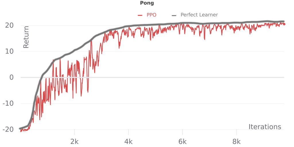
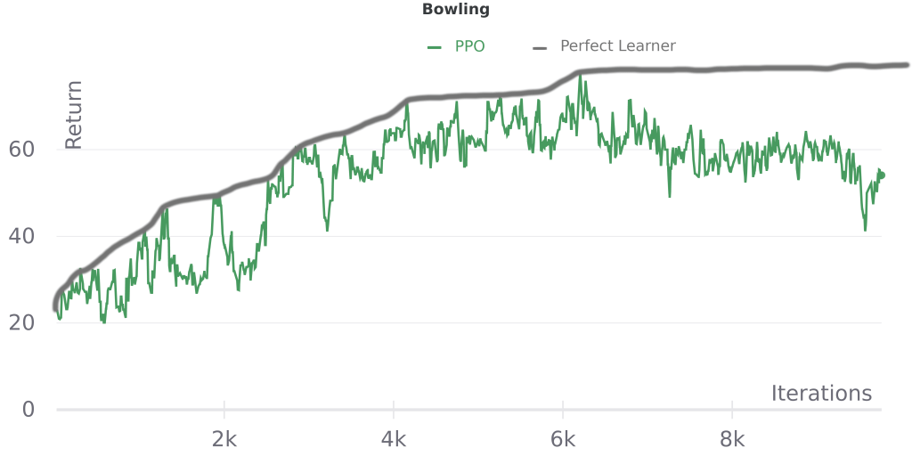
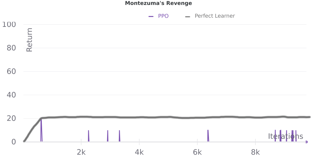
We can see that PPO is close to monotonic on Pong, which tracks with the general observation that most algorithms that build upon A2C/PPO don’t perform significantly better on this game. Meanwhile on Bowling PPO has more performance drops and it even declines late in training, consistent with recent work addressing the challenges caused by delayed rewards in that game. On Montezuma’s Revenge, we see that returns are mostly zero, and even a perfect learner would not perform well (returns can go much higher than 100), which fits with the idea that better sampling (exploration) is important for this game.

While simplistic, for tasks like these pick-the-max tracks with our intuition, so it’s worth considering whether it can be used for a new task before developing more sophisticated methods for domain-specific bottleneck detection.

Intra-MDP Generalization: Novelty Detection

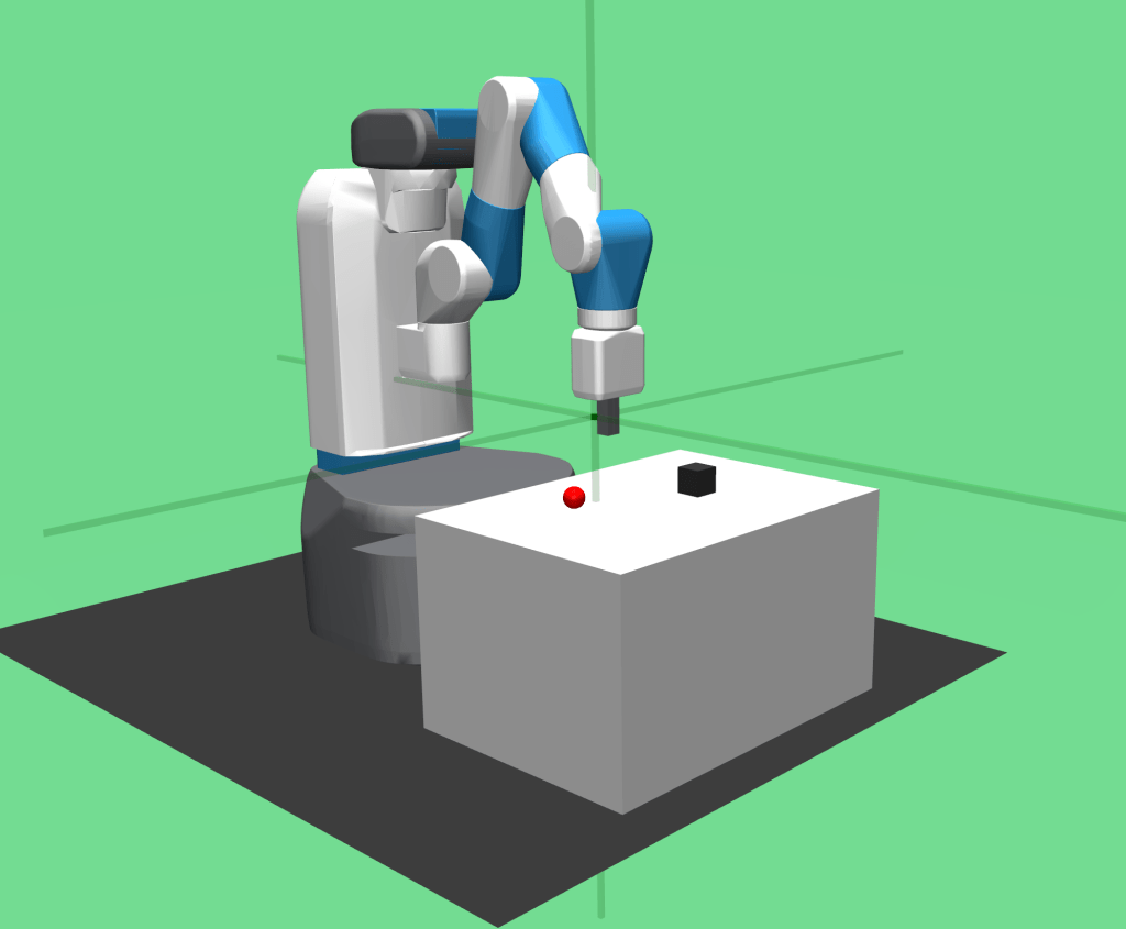
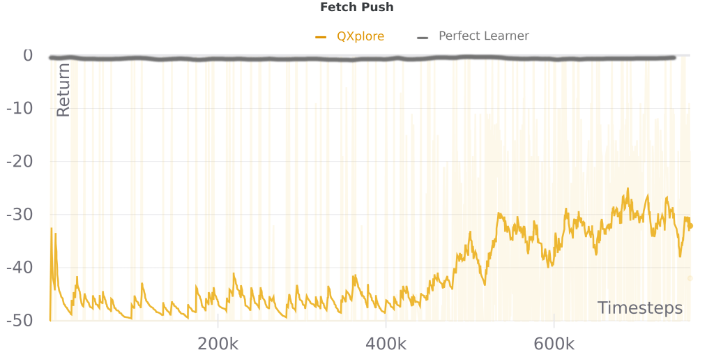
So where doesn’t pick-the-max make sense? When generalization comes into play*. Consider an MDP in which the agent starts out in a new part of the state space each episode which it is unlikely to have seen, but where the task/reward function and transition matrix remain the same. If the agent can’t generalize easily to the new initial condition, we can’t really expect our agent to match it’s previous performance- consider the FetchPush task, where a robot is tasked with pushing a block to a target position, with the block and target positions changing each episode. If our robot got lucky with easy positioning in its first episode, we can’t expect it to then generalize to all possible positions immediately.

How to handle this case? Our sampling strategy now needs to do two things: It needs to sample data suitable for learning a given subtask, while also sampling data that allows the agent to generalize to new subtasks. If we assume we never see the exact same subtask twice (reasonable for FetchPush and other cases, such as real world robotics), the generalization problem dominates, so the question becomes, how do we estimate the generalization difficulty of a new subtask given what the agent has previously sampled?

Unsurprisingly, this is hard in general. One approach is to estimate how “novel” fresh observations are- if they look nothing like what we’ve seen before, it’s (sometimes) reasonable to assume that we can’t generalize to them. While counterexamples abound (small perceptual changes with big effects, large changes that are irrelevant), this approach is convenient because we can borrow techniques from exploration- novelty metrics have been the subject of much study in that field.

Simple Model Error as a Generalization Upper Bound

While there’s a number of different approaches to computing perceptual novelty, the one I’m most familiar with is using model error. There’s an interesting quirk of neural networks that a number of papers have exploited (such as one of my own) wherein a network trained on a set of inputs S will smoothly deviate from the target value when given inputs that are numerically distinct from previously seen data.

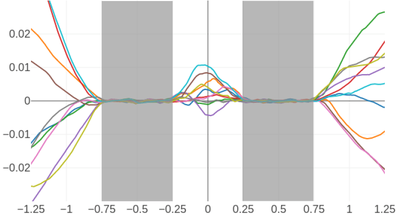
This property can be used as a measure of the “novelty” of a state. If our model of a simple function like f(s) = 1 is accurate for a given state s, then (in theory) the policy could also be accurate for a more complex function pi(s) = y.

In cases like the FetchPush example where returns are either 0 or 1 and state transitions are deterministic*, it’s reasonable to assume a policy overfit to a specific initial state can reliably obtain a return of 1. If our novelty model has error on a new subtask, this gives us a measure of how well we expect a policy that has mastered all previous subtasks to perform on this one.

Of course, this approach also has shortcomings- it assumes that the policy’s expected return will vary smoothly as one interpolates between states, and it’s easy to find counterexamples where numerically small changes in state result in large changes in dynamics, and thus a very different policy. For applications like robotic grasping, however, it might be a reasonable proxy for generalization to a new initial state.

More sophisticated methods, such as explicitly modeling the distribution over observed states and measuring the likelihood of new samples under that distribution might also work here. To do that one needs a good way to explicitly model the state distribution, which for complex observations like real-world images is not trivial. A lot of work has been done on unsupervised learning and generative modeling that might be useful for such an approach.

What about Stochastic MDPs?

Thus far I’ve outlined a couple of approaches for deterministic MDPs, but neither will work well if the environment or reward function is stochastic.

For example, consider the classic FrozenLake tabular MDP:

SFFF       (S: starting point, safe)
FHFH       (F: frozen surface, safe)
FFFH       (H: hole, fall to your doom)
HFFG       (G: goal, where the frisbee is located)

The agent starts at position S, and must navigate on the grid to G while avoiding holes H. The tricky part of this is that with every step there is a chance of moving a 90-degree rotation to the left or right of your intended movement direction (so trying to move down might move left or right with 10% probability each).

In this case, just because we saw the goal once doesn’t mean we know the optimal path- we might have simply gotten lucky, and repeating that path might only succeed a small fraction of the time. In a tabular MDP like this, we could of course simply compute the analytic policy gradient given some trajectory, which lets us compute the sampling regret, but this doesn’t work for deep RL.

So what does work? I’ve got a few imperfect ideas: If we know the success rate of the optimal policy (for FrozenLake it’s 1.0 given an infinite number of timesteps with no time decay on rewards, otherwise around ~0.6-0.7 with limited time or a decay horizon), we could use a modified take-the-max strategy by replaying the actions sampled in each episode multiple times to evaluate the true quality of that policy, but this is very inefficient and multiplies the number of interactions needed. Similarly, we could train an offline RL agent on data collected online and use its policy given unlimited training iterations as an estimate of the ideal learner, but this will be a very conservative estimate at best since offline RL is also an imperfect learning process.

Final Thoughts

As I said at the beginning, it’s difficult if not impossible to define a perfect measure of how sampling limits an RL agent. The ideas here outline some directions for possible imperfect measures, but there’s more that could be done. Stochasticity in particular remains an issue, and I welcome ideas for how to handle it better.

It’s also worth noting that there are more specific quantities we could measure besides sampling regret, which might also be useful. For example, we could compute metrics for the “exploration-hardness” of a problem based on agent performance, using things like the magnitude of the loss/gradient induced by a given batch of new data as a proxy its novel information content. For this blog post I opted to focus on a more universal measure, since this hasn’t really been mapped out before to my knowledge, but there are also specific bottleneck types that are common enough to be worth addressing individually (I might talk about these in the future, let me know if you’re interested!).

Some of the discussion around sampling regret is also relevant to the other regret measures I defined, which are useful for assessing how limiting RL algorithms or model architectures are. I’ll touch on this more in the next blog post in this series.

---

Footnotes:

^ For a given agent with given learning algorithm, hyperparameters, etc. This also glosses over the question of robustness- for a deterministic environment, the “perfect dataset” is simply one demonstration of the optimal trajectory, with the optimal agent simply imitating that trajectory exactly.

^ For example, if we are training a robot arm to pick up objects, with a return of 1 meaning a successful pickup and 0 meaning failure, we know that the optimal policy’s expected return should be (very close to) 1, so we can actually compute the regret during training. Similarly, we know for many Atari games what a perfect score is (such as Pong, where a score of 21 is perfect) or can define a score that is practically perfect (Montezuma’s Revenge has a fixed set of unique levels which repeat in order and a total score for clearing all unique levels).

^ Note that achieving 0 sampling regret is infeasible, we just want to minimize it.

^ This ignores exploration versus exploitation tradeoffs, but we could assume our ideal learner is strictly an exploitation policy, with a separate exploration policy to sample training data for it.

^ Whether the real world can be considered deterministic or not is a topic for another day. Suffice to say from the perspective of a robot who is the only active agent in its environment this is probably a reasonable approximation.

^ The PPO line in these plots shows the mean of the last 10 episodes, so the area under the perfect learner curve should be slightly larger, though the relative shapes of the two curves will be unchanged. This estimate also doesn’t account for run-to-run variance due to sampling, so ideally we’d average perfect learner performance across multiple runs.

^ Generalization is interesting here since it arguably straddles all three aspects: it depends heavily on what data you have (sampling), can be improved by specific model architectures (dimensionality reduction), and you can design learning rules that generalize better (e.g. Conservative Q-learning). I’ll talk more about this in a future blog post, since it’s a big topic deserving its own treatment.