
Summary
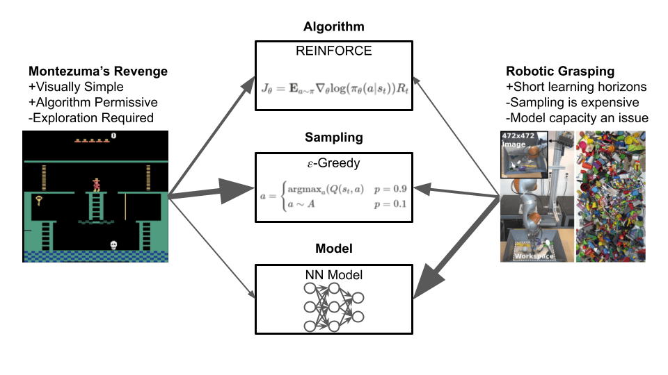
- Deep RL agent performance depends on three aspects of the agent: Update Algorithm, Sampling Strategy, and Model Architecture
- There’s evidence that for a given RL agent on a given MDP, one of these three will bottleneck performance
- Improving an aspect that isn’t a bottleneck will result in modest performance gains
- Conversely, improving an aspect which is a bottleneck will result in much larger gains
- There’s currently no good way to detect bottlenecks from common performance metrics
- In follow-up blog posts, I will discuss some possible ways to address this
Introduction
Hello and welcome to my blog! I’m starting this project with two goals in mind: First to practice writing technical material in more casual/accessible language (an important skill for any scientist), and second as a place to develop some ideas I’ve got kicking around that are interesting and novel, but not sufficient for proper peer-reviewed papers. Hopefully you find them interesting!
Today I’m starting a series of posts on learning bottlenecks in deep reinforcement learning. In this post I’ll describe the problem and some examples of how it expresses itself, with follow-on posts that go into more details on bottlenecks in specific aspects of an RL agent and how they can be resolved.
What is a Bottleneck?
One of the most unique elements of deep RL compared to most other domains of modern ML is how wildly an RL agent’s performance can vary between tasks, even for superficially similar ones. For example, consider the following performance plots from PPO:
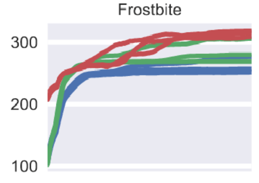

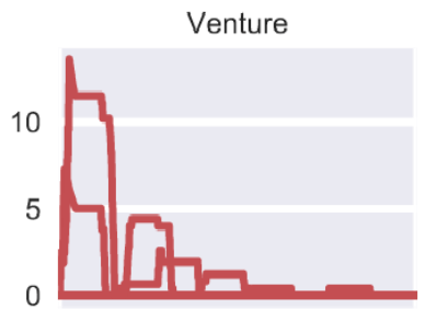
Running the same agents, with the same training process, on three different Atari games, results in huge differences in the delta between methods:
- On Frostbite, PPO (red) outperforms ACER (green) and A2C (blue) by a small amount, but all three methods plateau around the same reward level.
- On Kangaroo, PPO outperforms the same two methods by a huge margin- the performance of A2C and ACER on this game is around 50, indistinguishable from 0 compared to PPO’s 10,000+
- On Venture, none of the methods do well, final scores are around 0 for all three
So what’s the difference? Human performance is much better than A2C on all three of these games, so there’s room for improvement. The relative performance of a given RL agent will depend on the MDP, and some environments will be harder or easier for certain algorithms versus others. But what makes relatively similar (same observation/action spaces, same visual complexity, etc) MDP’s like these harder or easier?
Well, let’s consider how PPO differs from A2C. PPO modifies specific elements of A2C, namely how advantages are computed (generalized advantage estimation), constrains the policy gradients (via its clipped surrogate objective), and modifies the way gradient steps are taken (multiple epochs of minibatches)*. Meanwhile, PPO uses the same sampling strategy (stochastic policy plus entropy bonus) and model architecture (small CNN) as A2C.
Let’s next look at the three games from above:

In Frostbite the agent must jump between floating platforms to score points and build an igloo on the right side of the screen (shown completed above). Entering the igloo once built advances to the next level and scores many points, and while PPO (in my experience) sometimes samples this, none of the three agents do it reliably. PPO is more efficient at learning to maximize points from jumping on the platforms, but doesn’t learn to enter the igloo. The issue here is one of sampling- if PPO rarely observes the result of entering the igloo, it is unlikely to shift the policy enough to reliably sample it in the future*.
In Kangaroo, the agent controls the kangaroo at the bottom, who must reach the top level and collect fruit to score points, while dodging hazards dropping from above and defeating enemies that move horizontally. Discovering sources of reward is not difficult, but many different factors must be considered (hazards approach from multiple directions, the kangaroo is vulnerable while climbing ladders, etc) on long-ish time horizons, and A2C struggles to compute a stable policy gradient that improves the agent’s performance. PPO improves the quality of the computed gradient and allows for steady improvement.
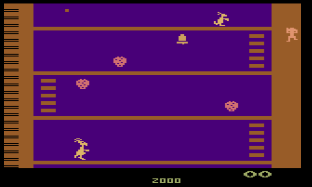
In Venture, the agent (the purple pixel at the bottom) must evade enemies and enter buildings (containing more enemies) to collect treasures, which are the sole source of points. Sampling any of the treasures at random is improbable due to distance and hazards, and as such all three algorithms rarely observe reward and thus fail to learn any policy better than random. A specific type of sampling behavior, long-range exploration, is needed to make this game tractable.
The common theme among the three is that each environment has specific challenges that stress different aspects of the RL agent. The improvement PPO provides on top of A2C helps with Kangaroo, but doesn’t address the core limitation in Frostbite and thus can only improve modestly. Meanwhile Venture requires heavyweight exploration to get anywhere, and thus PPO has no effect.
What can we do about this?
In this blog post, I’m going to lay out my hypothesis that different MDPs stress different elements of an RL agent, and that detecting which element is the bottleneck can help guide research in the field. These bottlenecks can be broken down into three broad categories: Those limited by the agent’s update rule (e.g. PPO), those limited by the agent’s sampling strategy (e.g. epsilon-greedy, exploration algorithms), and those limited by the agent’s model architecture (e.g. DQN’s 5-layer conv+FC network).
Succinctly put, The rate at which an RL agent improves on a given task will be limited (bottlenecked) by one of these three aspects at any given time. If we improve upon the limiting aspect, we will see large performance gains.
This might seem like an obvious point, but targeting which aspects of an algorithm to improve is a fundamental challenge in research- If we knew what was most fruitful to work on at all times, we’d progress much faster as a field. Making RL methods work for a given task is often more art than science, with lots of expert “black magic” required, and while there’s no silver bullet to address this, developing methods for identifying the weaknesses of RL algorithms can help to focus RL research and to make applied RL less of a dark art.
My hope in writing this blog post is to raise a little awareness around this issue, because it feels like often in RL we develop new algorithms without a strong prior that the task domain we’re interested in will significantly benefit from them (I’m guilty of this as well), and applying RL to solve problems is excessively ad-hoc and often relies on careful parameter tuning and task-specific hacks. Developing tools that can guide RL research should help both researchers and practitioners spend their time more efficiently and reduce the headaches of RL development.
There’s also an analogy to supervised learning that might aid understanding here: The three aspects of RL, algorithm, sampling, and model, are analogous to loss function, dataset, and network architecture from supervised learning.
Interestingly, in most domains of supervised learning more/better data (sampling) has led to major performance gains, and this is true for RL as well- with enough episodes a well-tuned REINFORCE implementation can probably reach high performance for most Atari games.
However, the interactive nature of RL means that just relying on more episodes/iterations doesn’t scale well, since it has to be repeated for every agent on every task. In domains of supervised learning where collecting more data is difficult, or where the field uses a fixed benchmark dataset for training and evaluation (e.g. Imagenet), we also see lots of work innovating on loss functions, model architectures, and data cleaning (“smart” sampling).
So the question then is, how can we identify what the bottleneck is for a given task?
This is sadly not simple to answer. The ways an RL agent can bottleneck are diverse, and there’s many ways bottlenecks can express themselves. There is no single solution. That said, I think we can define some general metrics that will at least cover the major pitfalls. In the following section I’m gonna go over a couple of example bottlenecks and how they fit into the three aspects, and then discuss some ideas for how they can be addressed in follow-up blog posts.
Sampling: Exploration
Probably the best known type of RL bottleneck is the exploration problem, which has been studied extensively, and is one type of sampling bottleneck.
The exploration problem, broadly put, covers situations in which an agent cannot improve in a reasonable amount of time by sampling experiences according to a stochastic return-maximizing policy. Examples of classic exploration-centric games in the Atari benchmark include Montezuma’s Revenge and Venture, though every MDP requires some measure of exploration (but simple methods might be good enough, depending).
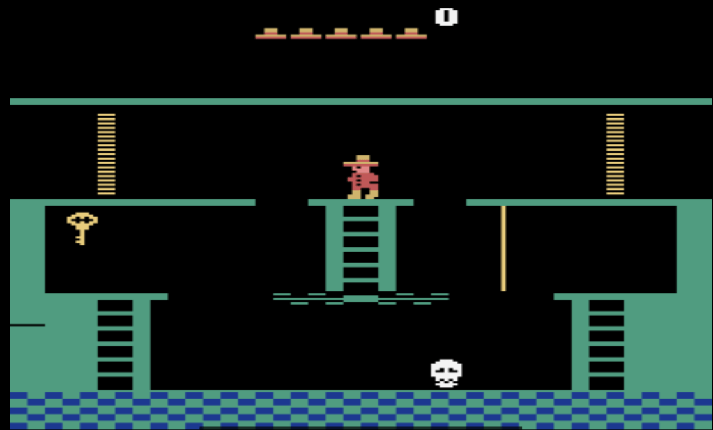
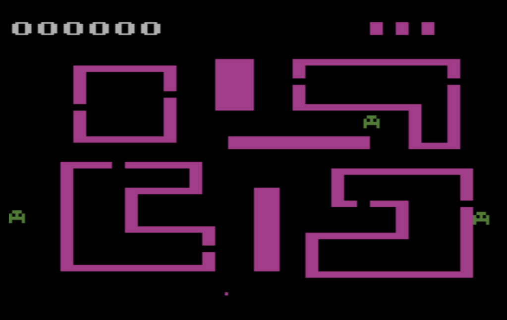
The key thing that makes these games hard for an agent like PPO is the reward function- in Montezuma’s Revenge, the agent controls the man wearing the hat, and to obtain the first non-zero reward in the game it must navigate to the key while avoiding long drops and the moving skull at the bottom, which will reset the agent’s position and lose one of 5 lives, after which the episode is over. This is all but impossible to do through the random actions an untrained policy will produce.
Similarly, in Venture, the agent controls the small dot at the bottom, and must enter the 4 rooms and evade enemies inside them to collect treasures, which are likewise the only sources of reward in the game.
In cases like these, the issue is one of sampling– the learning algorithm is capable of optimizing a policy to reach these goals, and the typical neural network models used are sufficient to fit that policy and any auxiliary functions. Improving the learning algorithm, as PPO does, provides little benefit on these games (though it does improve things slightly) because it’s not the bottleneck.
In addition to long-range exploration, sampling can also be an issue on a shorter time horizon- it’s easy for RL agents to get stuck in local return maxima like the one in Frostbite, where PPO converges to the local maxima of constructing the igloo, but doesn’t reliably enter the igloo despite that transition being discoverable without special long-range exploration techniques.
Let’s look at an example of an algorithm bottleneck I encountered in my own recent work: Credit Assignment.
Algorithm: Credit Assignment
Briefly put, the credit assignment problem in RL can be stated as “how did my action at time t affect the reward I got at time t+k?” While every RL agent must learn this relationship somehow, most of the time it is learned through correlations– the agent samples many different actions (with similar actions in the span of time between t and t+k) and at the end of it discovers that some action a is correlated with a (hopefully large) reward r in the future.
The downside to this approach is of course that correlation is not causation- RL agents can (and in practice do) pick up behaviors that happened to spuriously correlate with high reward but are ultimately unrelated to it. These spurious correlations can also slow down learning, as they may incentivize behaviors that prevent achieving even higher rewards.
I recently wrote a paper on this topic, where we proposed a method for using explicit credit assignment that captures the mutual information (rather than just correlation) between actions and future states/rewards. I won’t get into the details here, but in principle this seems like a good idea- we learn an additional piece of information relevant to the task which can be directly used to learn a better policy, and we devised a clever way to avoid issues stemming from limited training data/bias in the explicit credit model. Thus, we expected to see “generally better” performance on most tasks.
The reality of it is slightly more complicated- I’ve included the performance plot of performance versus our credit assignment hyperparameter* from the paper below. This example is nice because C2A2C (our method) only modifies the update rule for A2C- it preserves the network architecture and sampling behavior entirely, so any effects it has can be attributed to the policy gradients computed. One surprising finding is that while there’s always a hyperparameter for C2A2C that doesn’t make performance worse compared to A2C (and we have ideas for how to improve the method to prevent bad hyperparameter settings degrading performance), the performance gains were concentrated on a handful of games- most of the Atari games we tested didn’t benefit much from better credit assignment. However, a subset of games saw much better performance, double or more the baseline.
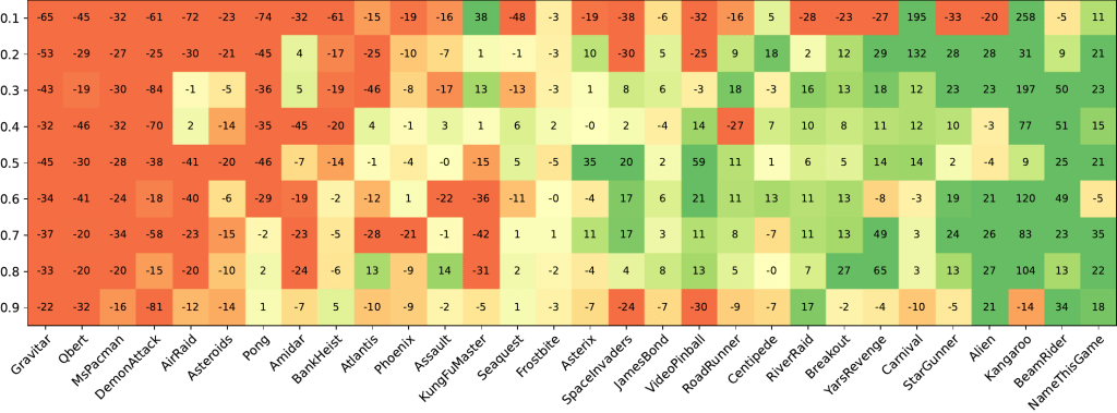
Our intuition before doing large-scale experiments was that we expected to see modest-but-consistent gains across most games, but the evidence suggests that credit assignment is particularly important for a subset of games*, while others are largely indifferent. Let’s look at one of the biggest standouts, Carnival:
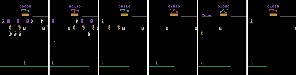

Carnival is a shooting gallery- the agent controls the gun at the bottom, and must hit all targets (plus the windmill at the center top, which ends the episode when shot) with a limited amount of bullets. Credit assignment is tricky here because bullets have travel time, during which the agent can keep shooting- The agent might fire bullets that miss while bullets that hit a target are in the air, and thus learn a spurious correlation between the two.
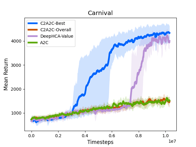
A2C does okay at this game- it learns to avoid hitting the windmill by sticking to the corner to avoid prematurely ending the episode, but in doing so limits how many points it can obtain. C2A2C on the other hand seems to learn the difference between shooting the windmill and shooting other targets nearby, and discovers that it’s okay to shoot the windmill once the other targets are gone. This results in much higher scores on this game.
The point of all this is that the specific characteristics of Carnival (and Kangaroo, BeamRider, Video Pinball, etc.) meant better credit assignment resulted in better performance, whereas most Atari games didn’t see much benefit from it- the correlation-based credit assignment used by A2C was sufficient for those games (though other algorithmic improvements might still help).
Detecting Bottlenecks
Now for the million-dollar question: If different tasks will benefit from different algorithmic changes, how do we tell what changes an environment will actually benefit from?
In an absolute sense, this is hard- edge cases are common in RL, and many a paper contains a constructed test MDP where the proposed algorithm is needed for the agent to learn. That said, some types of bottlenecks (such as exploration) appear in many tasks, meaning that techniques for detecting them should be broadly useful.
One caveat to keep in mind in considering this question is that there’s no free lunch here- any metric we use to detect bottlenecks will be biased or otherwise heuristic. There will be cases where our metric gives a misleading signal. That said, in my mind the question is not whether we can define a perfect measure of (for example) the credit-assignment-hardness of an MDP*, but whether the metric of credit-assignment-hardness we define is useful for RL research or deployment. Can we save valuable time and headache by helping RL researchers identify the problems most in need of solving for a given MDP?
This is a broad question, and I don’t expect to cover all possible things we’d like to measure on this blog. In follow-on blog posts, I’m gonna cover some of what I think are the most tractable metrics for common bottlenecks. My aim is to release 3 posts, one covering metrics related to each of the core RL agent aspects (algorithm, sampling, model). The first of these, on sampling, should go up shortly after this introductory post so as to not draw out the suspense too long. 🙂
Footnotes:
^ PPO Also modifies several hyperparameters (e.g. the length of bootstrapped rollouts), which will affect performance along different axes, but the major contributions of the paper center around how policy gradient updates are made and it’s IMO reasonable to attribute most of the performance increases to those.
^ Alternately, this could be treated as a problem of learning from very few examples (an algorithm bottleneck), given that PPO will occasionally enter the igloo but rarely if ever do so reliably, but for an on-policy algorithm it’s probably easier to address via sampling.
^ This parameter determines how conservative to be about assigning credit- 1.0 is equal to A2C, while 0.1 means only 10% of actions are credited. Games where most actions should be credited want high values and benefit only a little from values less than 1, while games where most actions shouldn’t be credited (because that would slow/prevent policy improvement) prefer low values close to 0.
^ Other standouts that benefit include Kangaroo, though C2A2C doesn’t improve over A2C as much as PPO does, and performance is highly sensitive to specific credit hyperparameter values. Personally I suspect the two combined would be better than each individually since PPO doesn’t really address the correlation-versus-causation question and it seems there’s enough undesirable action-return correlations (for example, punching enemies scores points but makes it harder to dodge projectiles as the kangaroo can’t move while punching) for C2A2C to help.
^ I suspect a perfect measure is impossible, at least outside tabular MDPs, though I’d be happy to be proven wrong!
